
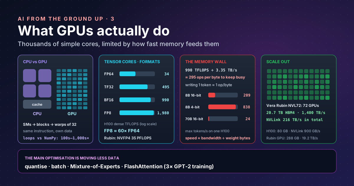
Part 1 showed that an LLM is mostly matrix multiplication: about 2 × n³ multiply-and-add operations for two n × n matrices, and nearly every one of them independent of the others. This part is about the hardware built to do exactly that, and the one limit that surprises most people: memory, not arithmetic.
Why not a CPU?#
NVIDIA’s own CUDA programming guide puts the difference in one sentence: GPUs “devote more transistors to data processing units, while CPUs dedicate more transistors to data caching and flow control”.
| CPU | GPU | |
|---|---|---|
| Cores | A few to a few hundred, each powerful | Thousands of simple ones |
| Good at | Branching logic, one task fast (latency) | The same operation on lots of data (throughput) |
| Chip area spent on | Caches, branch prediction, out-of-order tricks | Arithmetic units |
| AI fit | Orchestration, data loading, small models | Training and serving large models |
You can feel the difference without a GPU. The same 200 × 200 matrix multiplication, done one operation at a time in plain Python, and then handed to NumPy, which uses optimised code that works on many numbers at once:
import time
import numpy as np

n = 200
A, B = np.random.rand(n, n), np.random.rand(n, n)

def matmul_loops(A, B):                      # one multiply-add at a time, like a single worker
    C = [[0.0] * n for _ in range(n)]
    for i in range(n):
        for j in range(n):
            s = 0.0
            for k in range(n):
                s += A[i, k] * B[k, j]
            C[i][j] = s
    return C

t = time.perf_counter(); matmul_loops(A, B); loops = time.perf_counter() - t
t = time.perf_counter(); A @ B; vec = time.perf_counter() - t
print(f"{n}x{n} matrix multiply: {2 * n**3:,} operations")
print(f"Python loops: {loops:.2f} s")
print(f"NumPy (vectorised, many cores, SIMD): {vec * 1000:.2f} ms  ->  {loops / vec:,.0f}x faster")
On my laptop:
200x200 matrix multiply: 16,000,000 operations
Python loops: 1.37 s
NumPy (vectorised, many cores, SIMD): 0.81 ms  ->  1,687x faster
Same arithmetic, hundreds to thousands of times faster, just by doing many operations at once. Timings this short are noisy: a second run on the same laptop gave 663×, so treat the number as an order of magnitude. A data-centre GPU takes the same idea several orders of magnitude further.
Inside a GPU: thousands of workers in lockstep#
The CUDA programming model describes the structure from the top down:
- A GPU is “a collection of Streaming Multiprocessors (SMs)”, each a small processor with its own cores and fast local memory.
- A program for the GPU (a kernel) is launched as a grid of thread blocks; “all threads of a thread block are executed in a single SM”.
- Inside a block, “threads are organized into groups of 32 threads called warps”, and a warp executes in a “Single-Instruction Multiple-Threads (SIMT) paradigm”: all 32 run the same instruction, each on its own data.
So a matrix multiplication is split into tiles, each tile goes to a block, and every thread computes a few output
numbers. Because the threads of a warp share one instruction stream, code that branches differently per thread
wastes the hardware, which is why GPU code avoids if statements in hot loops and why AI frameworks ship
hand-tuned kernels rather than asking you to write them.
Tensor cores and small numbers#
Modern GPUs add tensor cores: units that multiply whole small matrices in one step instead of one pair of numbers at a time. They are fastest with fewer bits per number, and that is where most of the headline speed comes from. NVIDIA’s H100 page shows it plainly:
| Number format (H100 SXM) | Throughput listed | Without sparsity* |
|---|---|---|
| FP64, 64-bit (scientific computing) | 34 TFLOPS (67 on tensor cores) | same |
| TF32 tensor core | 989 TFLOPS* | about 495 |
| BF16 / FP16 tensor core, 16-bit | 1,979 TFLOPS* | about 990 |
| FP8 tensor core, 8-bit | 3,958 TFLOPS* | about 1,980 |
*The page marks tensor-core figures “with sparsity”, a feature that skips zeros in a specific pattern and doubles the number; dense work gets about half. Even so, the jump from FP64 to FP8 is roughly 60-fold.
LLMs tolerate low precision well, so training runs in 16 or 8 bits and serving often in 8 or 4. That is why model cards talk about FP8 weights and INT4 quantisation: fewer bits mean more operations per second and, as the next section shows, less memory to move.
The memory wall#
Arithmetic is cheap; moving data is not. A GPU keeps the model in HBM (high-bandwidth memory) stacked next to the chip, and every number must be read from HBM into the cores before it can be used.
A useful way to see the limit is arithmetic intensity: operations done per byte read. On an H100:
990 trillion operations per second ÷ 3.35 trillion bytes per second ≈ 295 operations per byteIf your work does fewer than about 295 operations for every byte it reads, the cores sit idle waiting for memory: the job is memory-bound. Above that, it is compute-bound.
Why generating text is memory-bound#
When a model writes an answer for one user, each new token needs every weight once, and each weight is used for only about two operations (one multiply, one add). Two operations per two bytes of a 16-bit weight is an intensity near 1, hundreds of times below the ridge point. So the speed limit is simply how fast the weights can be streamed from memory:
# Upper bound on single-user generation speed when every token must read all the weights once
def max_tokens_per_second(params_billion, bytes_per_param, bandwidth_tb_s):
    model_bytes = params_billion * 1e9 * bytes_per_param
    return bandwidth_tb_s * 1e12 / model_bytes

for name, p, b in [("8B model, 16-bit", 8, 2), ("8B model, 4-bit", 8, 0.5), ("70B model, 16-bit", 70, 2)]:
    print(f"{name:<18} on H100 (3.35 TB/s): at most {max_tokens_per_second(p, b, 3.35):5.0f} tokens/s")
8B model, 16-bit on H100 (3.35 TB/s): at most 209 tokens/s
8B model, 4-bit on H100 (3.35 TB/s): at most 838 tokens/s
70B model, 16-bit on H100 (3.35 TB/s): at most 24 tokens/sThis back-of-the-envelope sum explains a lot of real behaviour:
- Quantisation speeds up answers mainly because there are fewer bytes to read, not fewer sums to do.
- Batching is how providers make serving affordable. Reading the weights once and using them for many users' tokens raises the intensity towards the ridge point.
- Mixture-of-Experts helps: only the active experts’ weights are read per token.
- Long contexts slow things down, because the KV cache (part 1) must be read for every new token too.
Training is different: huge batches reuse each weight many times, so it is usually compute-bound, and that is where the tensor-core numbers matter.
Keeping data close: FlashAttention#
Each SM also has a small, very fast on-chip memory (SRAM). The FlashAttention paper showed that standard attention wasted time “reads and writes between levels of GPU memory” and, by computing attention in tiles that stay in SRAM, trained GPT-2 about 3× faster with exactly the same result. Much of modern AI performance work is like this: not new maths, but less data movement.
One GPU is not enough: scaling out#
A trillion-parameter model does not fit on one GPU (H100 has 80 GB), so many GPUs work as one. That needs fast links between them: H100’s NVLink moves 900 GB/s, far faster than ordinary networking, and racks join dozens of GPUs into one domain. The How an LLM is built series shows how Kimi K2 split its training three ways (pipeline, expert and data parallelism) across thousands of H800s.
Today’s numbers, from H100 to Rubin#
NVIDIA’s current generation is Rubin, sold as the Vera Rubin NVL72 rack, which the product page says is “now in full production”:
| H100 SXM | Rubin GPU | Vera Rubin NVL72 rack | |
|---|---|---|---|
| Memory | 80 GB | 288 GB HBM4 | 20.7 TB HBM4 |
| Memory bandwidth | 3.35 TB/s | 19.2 TB/s | 1,400 TB/s |
| Low-precision training (dense) | FP8 ≈ 1,980 TFLOPS | NVFP4 35 PFLOPS; FP8 17.5 PFLOPS | NVFP4 2,520 PFLOPS |
| GPU-to-GPU link | NVLink 900 GB/s | NVLink 3 TB/s | 216 TB/s in total |
| GPUs | 1 | 1 | 72 (with 36 Vera CPUs) |
Memory bandwidth grew almost six-fold from H100 to Rubin, and dense FP8 training about nine-fold. The trend is clear in the design: more memory, faster memory, smaller numbers (FP4), and more GPUs joined into one rack-sized machine.
Do you need a GPU?#
| You want to | You need |
|---|---|
| Use a hosted model through an API | No GPU at all |
| Run a small open model (a few billion parameters) | A laptop GPU or Apple silicon is enough; see Ollama |
| Fine-tune a model with LoRA | One or a few rented data-centre GPUs |
| Serve an open model to many users | Several GPUs with lots of memory, and batching |
| Pre-train a frontier model | Tens of thousands of GPUs (part 4) |
Takeaways#
- GPUs win by doing thousands of simple operations at once, which is exactly what matrix multiplication needs.
- Tensor cores and low-precision numbers provide most of the speed; FP8 is about 60× FP64 on an H100.
- Generating text is usually memory-bound: speed is roughly memory bandwidth divided by the bytes of weights.
- Less data movement is the main optimisation, from quantisation and batching to FlashAttention.
- Big models need many GPUs joined by fast links; Rubin-generation racks join 72.
Keywords#
| Term | What it means |
|---|---|
| GPU | Graphics processing unit: a chip with thousands of simple cores for parallel work. |
| Latency / throughput | How fast one task finishes, versus how much work gets done per second. |
| SIMD / SIMT | One instruction applied to many pieces of data / many threads at once. |
| Streaming Multiprocessor (SM) | One of the GPU’s many small processors. |
| Kernel | A function that runs on the GPU. |
| Thread block / grid | A group of GPU threads that runs on one SM / all the blocks of one kernel launch. |
| Warp | 32 threads that execute the same instruction together. |
| Tensor core | A unit that multiplies small matrices in one step. |
| FLOPS | Floating-point operations per second (TFLOPS = trillions, PFLOPS = thousands of trillions). |
| FP64 / FP16 / BF16 / FP8 / FP4 | Number formats with 64, 16, 8 or 4 bits; fewer bits are faster and smaller but less precise. |
| Sparsity | Skipping zeros in a fixed pattern; doubles the listed tensor-core speed. |
| Quantisation | Storing weights in fewer bits to save memory and time. |
| HBM | High-bandwidth memory stacked next to the GPU chip. |
| SRAM | Tiny, very fast memory on the chip itself. |
| Memory bandwidth | Bytes per second the GPU can read from memory. |
| Arithmetic intensity | Operations done per byte read; below the ridge point the job is memory-bound. |
| Memory-bound / compute-bound | Limited by moving data / by doing arithmetic. |
| Batching | Processing many requests together so each weight read is reused. |
| NVLink | NVIDIA’s fast GPU-to-GPU connection. |
References#
- CUDA Programming Guide: Introduction: NVIDIA; GPUs devote more transistors to data processing, CPUs to caching and flow control
- CUDA Programming Guide: Programming Model: NVIDIA; SMs, kernels, thread blocks, grids, 32-thread warps and SIMT
- NVIDIA H100 Tensor Core GPU: NVIDIA; H100 SXM throughput by format, 80 GB memory, 3.35 TB/s bandwidth, NVLink 900 GB/s, and the sparsity footnote
- NVIDIA Vera Rubin NVL72: NVIDIA; Rubin GPU and NVL72 rack specifications and production status
- FlashAttention: Fast and Memory-Efficient Exact Attention with IO-Awareness: Dao et al. (arXiv); memory reads and writes as the bottleneck, tiling in SRAM, 3× faster GPT-2 training
Related: Matrix multiplication to GPUs and How an LLM is built, part 2: pre-training.