
Part 1 ended with softmax turning a model’s raw scores into probabilities. This part is about what those probabilities mean, how training uses them, and how they become the words you actually read. As before, every example runs with Python and NumPy, and I show the real output.
The few ideas you need#
| Idea | Plain meaning | Example |
|---|---|---|
| Probability | How likely something is, from 0 (never) to 1 (certain) | P(heads) = 0.5 |
| Random variable | A quantity whose value is uncertain | the next token, tomorrow’s error count |
| Distribution | The probabilities of every possible value, adding up to 1 | Paris 85%, London 7%, … |
| Conditional probability | How likely A is, given that B is known; written P(A | B) | P(rain | dark clouds) |
| Independence | Knowing B tells you nothing about A | two coin tosses |
| Expected value | The average outcome, weighting each by its probability | average loss over the data |
The most important row is conditional probability. Almost everything a model predicts is conditional: the probability of this label given this email, of this token given the text so far.
Bayes’ rule: updating a belief with evidence#
Bayes’ rule says how to update a belief when evidence arrives:
P(A | B) = P(B | A) × P(A) / P(B)In words: how likely the cause is given the evidence equals how likely the evidence is if the cause is true, times how likely the cause was to begin with (the prior), divided by how likely the evidence is overall.
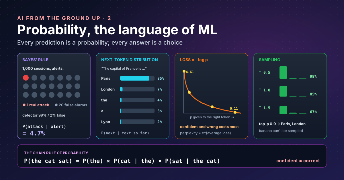
It matters because intuition gets it badly wrong. Take an intrusion detector that catches 99% of attacks and wrongly flags only 2% of normal sessions. An alert fires. How likely is a real attack?
# An alert fires. How likely is a real intrusion?
p_attack = 0.001            # prior: 1 in 1,000 sessions is an attack
p_alert_if_attack = 0.99    # the detector catches 99% of attacks
p_alert_if_normal = 0.02    # and wrongly flags 2% of normal sessions

p_alert = p_alert_if_attack * p_attack + p_alert_if_normal * (1 - p_attack)
p_attack_if_alert = p_alert_if_attack * p_attack / p_alert      # Bayes' rule
print(f"P(alert)          = {p_alert:.4f}")
print(f"P(attack | alert) = {p_attack_if_alert:.1%}")
P(alert) = 0.0210
P(attack | alert) = 4.7%Under 5%. Attacks are so rare that the 2% of false alarms on normal traffic swamp the real ones: in 1,000 sessions, about one alert is an attack and about twenty are not. This is the base-rate effect, and it is why every security team drowns in alerts. The same sum explains why a classifier with “99% accuracy” can be useless on rare events, and why you should look at precision and recall, not accuracy alone.
Bayes’ rule is also the oldest machine-learning trick in production: a naive Bayes spam filter multiplies the probability of each word given “spam” and given “not spam”, and applies the rule to decide.
An LLM is a probability machine#
Strip away the engineering and an LLM does one thing: given the text so far, it outputs a distribution over every token in its vocabulary for what comes next. For “The capital of France is”, that might be Paris 85%, London 7%, “the” 4%, and so on down a very long tail.
A whole sentence is a chain of these. By the chain rule of probability:
P("the cat sat") = P("the") × P("cat" | "the") × P("sat" | "the cat")The model never stores whole sentences. It only ever learns the next conditional step, and a sentence’s probability is the product of the steps.
Training is maximising probability#
Part 1 said training lowers a loss. For an LLM that loss is defined by probability: look at the probability the model gave to the token that actually came next, and take minus its logarithm. This is the cross-entropy loss (the negative log-likelihood):
import math
# The model gave the real next token this probability; the loss is -log(p)
for p in (0.9, 0.5, 0.1, 0.01):
    print(f"p(correct) = {p:<5} loss = {-math.log(p):.2f}   perplexity = {1/p:.1f}")
p(correct) = 0.9 loss = 0.11 perplexity = 1.1
p(correct) = 0.5 loss = 0.69 perplexity = 2.0
p(correct) = 0.1 loss = 2.30 perplexity = 10.0
p(correct) = 0.01 loss = 4.61 perplexity = 100.0Why the logarithm? Three reasons:
- It turns products into sums. The probability of a document is a product of thousands of small numbers, which would underflow to zero; the sum of their logs is well behaved.
- It punishes confident mistakes hard. Giving the right answer 1% costs 4.61; giving it 90% costs only 0.11.
- Minimising it is the same as maximising the probability of the training text (maximum likelihood).
Perplexity is the exponential of the average loss: roughly, how many tokens the model is “torn between” at each step. A perplexity of 10 means the model is, on average, as unsure as if choosing among 10 equally likely tokens. When the Kimi K2 training run shows a falling loss curve, this is the number falling.
From probabilities to words: sampling#
The model gives a distribution; something must pick one token. That choice is decoding, and it is where the settings you see in every AI product come in.
| Method | How it picks | Effect |
|---|---|---|
| Greedy | Always the most likely token | Repeatable, but can be dull and repetitive |
| Sampling | At random, in proportion to the probabilities | Varied; sometimes picks something odd |
| Temperature | Divide the logits by T before softmax | T < 1 sharpens the distribution, T > 1 flattens it |
| Top-k | Sample only from the k most likely tokens | Cuts off the long tail |
| Top-p (nucleus) | Sample from the smallest set of tokens whose probabilities add up to p | Adapts the cut-off to how sure the model is |
Why not always take the most likely token? Because, as the nucleus sampling paper put it, “using likelihood as a decoding objective leads to text that is bland and strangely repetitive”. Top-p was its answer: sample, but only from the reliable head of the distribution, “truncating the less reliable tail”.
Here are all three knobs on one made-up distribution:
import numpy as np

tokens = ["Paris", "London", "the", "a", "Lyon", "banana"]
logits = np.array([6.0, 3.5, 3.0, 2.5, 2.0, -1.0])   # the model's raw scores for the next token

def probs(logits, temperature=1.0):
    z = logits / temperature
    e = np.exp(z - z.max())
    return e / e.sum()

def top_p(p, threshold=0.9):
    order = np.argsort(p)[::-1]                    # most likely first
    keep = np.cumsum(p[order]) - p[order] < threshold   # smallest set reaching the threshold
    q = np.zeros_like(p); q[order[keep]] = p[order[keep]]
    return q / q.sum()

for t in (0.5, 1.0, 1.5):
    print(f"T={t}: " + "  ".join(f"{w} {x:.0%}" for w, x in zip(tokens, probs(logits, t))))
print("top-p 0.9 at T=1.0: " + "  ".join(f"{w} {x:.0%}" for w, x in zip(tokens, top_p(probs(logits))) if x > 0))

rng = np.random.default_rng(42)
draws = rng.choice(tokens, size=1000, p=probs(logits))
print("1,000 samples at T=1.0:", {w: int((draws == w).sum()) for w in tokens})
T=0.5: Paris 99% London 1% the 0% a 0% Lyon 0% banana 0%
T=1.0: Paris 85% London 7% the 4% a 3% Lyon 2% banana 0%
T=1.5: Paris 67% London 13% the 9% a 6% Lyon 5% banana 1%
top-p 0.9 at T=1.0: Paris 92% London 8%
1,000 samples at T=1.0: {'Paris': 846, 'London': 70, 'the': 42, 'a': 24, 'Lyon': 18, 'banana': 0}Read it as three lessons:
- Low temperature makes the model nearly deterministic; high temperature gives the tail a real chance. At 1.5, “banana” appears about once in a hundred tries.
- Top-p 0.9 throws away everything after Paris and London, so nonsense cannot be sampled at all.
- Sampling is random, so the same prompt gives different answers. 846 out of 1,000 were Paris, close to the 85% you would expect. If you need repeatable output, that has to be designed for; part 5 covers how.
Many products set these knobs for you, or hide them, but the mechanism underneath is the same.
Confidence is not correctness#
A probability is only useful if it is calibrated: when a model says 80%, it should be right about 80% of the time. A well-known study found that “modern neural networks, unlike those from a decade ago, are poorly calibrated”, usually overconfident, and that a one-number fix, temperature scaling, is “surprisingly effective” at repairing it.
For LLMs the lesson is practical. The probability of a token measures how typical the text is, not whether it is true. A fluent, confident wrong answer (a “hallucination”) is exactly what a probability machine produces when the most likely continuation is not the correct one. Checking facts against sources, as in RAG, exists because of this.
Where else probability shows up#
| In machine learning | The probability behind it |
|---|---|
| Classifiers (spam, fraud, sentiment) | P(label | input); a threshold turns it into a decision |
| Training loss | Cross-entropy: minus the log-probability of the right answer |
| Dropout and random initialisation | Deliberate randomness so the model does not over-fit |
| Splitting data, mini-batches | Random samples so each step sees a fair slice of the data |
| Evaluation | Results on a sample, with uncertainty: 95% on 40 questions is a weak claim |
| Monte Carlo methods | Estimating answers by repeated random trials (see my Monte Carlo post) |
Takeaways#
- Machine learning outputs probabilities; a decision rule (a threshold, a sampler) turns them into actions.
- Bayes’ rule beats intuition: with rare events, most alarms are false even from an accurate detector.
- An LLM predicts one conditional distribution at a time, and training maximises the probability of real text (cross-entropy loss, perplexity).
- Temperature and top-p decide how adventurous the chosen words are; sampling is why answers vary.
- Confident is not correct. Probability measures typicality, not truth.
Keywords#
| Term | What it means |
|---|---|
| Probability | How likely something is, from 0 to 1. |
| Distribution | Probabilities for every possible outcome, adding up to 1. |
| Conditional probability | P(A | B): how likely A is when B is known. |
| Prior | What you believed before seeing the evidence. |
| Bayes’ rule | How to update the prior with evidence to get P(cause | evidence). |
| Base rate | How common something is to begin with; ignoring it causes most false-alarm surprises. |
| Precision / recall | Of the alerts, how many were real; of the real cases, how many were caught. |
| Chain rule of probability | A sequence’s probability is the product of each step’s conditional probability. |
| Likelihood | How probable the observed data is under the model. |
| Cross-entropy / negative log-likelihood | Minus the log-probability of the right answer; the standard training loss. |
| Perplexity | The exponential of the average loss: how many tokens the model is effectively torn between. |
| Logit | A raw score before softmax. |
| Decoding | Choosing actual tokens from the model’s probabilities. |
| Greedy decoding | Always picking the most likely token. |
| Temperature | Divides the logits before softmax: below 1 sharper, above 1 flatter. |
| Top-k / top-p | Sample only from the k most likely tokens, or from the smallest set covering probability p. |
| Calibration | Whether stated confidence matches how often the model is right. |
| Hallucination | A fluent, confident answer that is false. |
References#
- The Curious Case of Neural Text Degeneration: Holtzman et al. (arXiv); why likelihood-maximising decoding is bland and repetitive, and nucleus (top-p) sampling
- On Calibration of Modern Neural Networks: Guo et al. (arXiv); modern networks are poorly calibrated, and temperature scaling fixes much of it
- Kimi K2: Open Agentic Intelligence: Kimi Team, Moonshot AI (arXiv); a real training run’s loss curve, referenced via part 2 of How an LLM is built
Related: AI from the ground up, part 1, The probability engine and Monte Carlo optimisation.