Why bother with the maths#
You can use an LLM without any of this. But the maths explains things you will meet every day: why models need GPUs (part 3), why answers change between runs (part 2), why a model can be “confidently wrong”, and why a bigger context costs more. It also makes the How an LLM is built series easier to follow.
This series has a short warm-up and five parts:
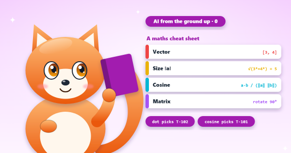
- A maths cheat sheet: vectors, norms, cosine and matrices, if they are new to you
- The maths behind an LLM (this post)
- Probability, and how machine learning uses it
- What GPUs actually do
- Frontier models, with examples
- Using models effectively
All the code here needs only Python and NumPy (pip install numpy). I ran every example on my laptop and show the
real output.
1. Vectors: meaning as a list of numbers#
A computer cannot compare the meaning of “cat” and “dog”. It can compare numbers. So every token (a word or piece of a word) is turned into a vector: a fixed-length list of numbers, called an embedding. Training adjusts those numbers until tokens used in similar ways end up with similar lists.
How do you measure “similar”? With the dot product: multiply the two lists position by position and add the results. If both lists are large in the same places, the sum is large. But a bigger list gives a bigger sum even when the meaning is no closer, so divide by each vector’s size (its norm: square every number, add them, take the square root). What is left is the cosine similarity, the cosine of the angle between the two arrows: from −1 (opposite) through 0 (unrelated) to 1 (same direction). It compares direction only, and direction is where an embedding keeps meaning. (New to vectors and norms? The maths cheat sheet covers them, with a worked example.)
import numpy as np

# Toy 4-number "meanings" (real models learn thousands of numbers per token)
words = {
    "cat":   np.array([0.9, 0.8, 0.1, 0.0]),
    "dog":   np.array([0.8, 0.9, 0.2, 0.0]),
    "pod":   np.array([0.0, 0.1, 0.9, 0.8]),
    "node":  np.array([0.1, 0.0, 0.8, 0.9]),
}

def cosine(a, b):
    return a @ b / (np.linalg.norm(a) * np.linalg.norm(b))   # @ is the dot product

for a, b in [("cat", "dog"), ("pod", "node"), ("cat", "node")]:
    print(f"{a:>4} vs {b:<4} similarity {cosine(words[a], words[b]):.2f}")
cat vs dog similarity 0.99
pod vs node similarity 0.99
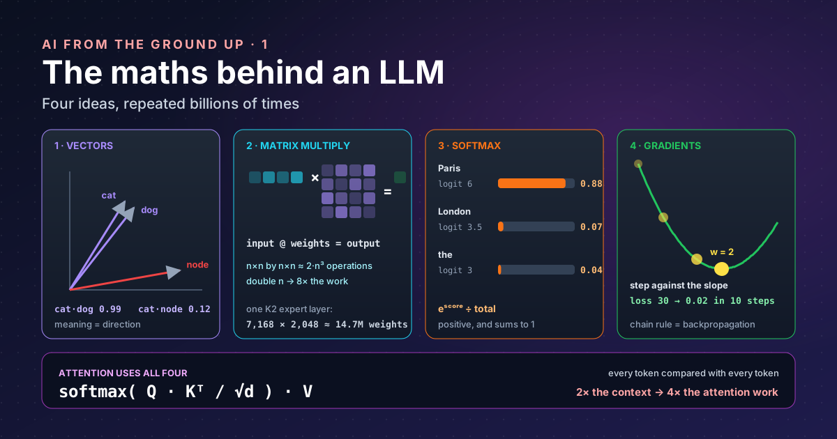
cat vs node similarity 0.12I made up those numbers so the pets and the Kubernetes words land apart. A real model learns them, and uses far more of them: the Kimi K2 model gives every token a vector of 7,168 numbers. The same dot product powers semantic search and RAG: turn the question and the documents into vectors, and fetch the documents whose vectors point the same way.
2. Matrix multiplication: the workhorse#
A matrix is a grid of numbers. Multiplying a vector by a matrix produces a new vector, and every number in the
result is a dot product of the input with one column of the matrix. That is all a neural network layer does at
heart: output = input @ weights, followed by a simple bend such as “replace negatives with zero” so that stacked
layers can learn curves, not just straight lines.
The weights are the model’s parameters: the numbers training adjusts. A single 7,168 × 2,048 weight matrix (the size of one expert’s layer in Kimi K2) already holds about 14.7 million of them, and the model has thousands of such matrices.
Multiplying an n × n matrix by another takes about 2 × n³ operations (n³ multiplications and n³ additions). Double the size and the work grows eightfold. Nearly all the time an LLM spends, in training and in answering, is spent here, which is why part 3 is about hardware built for exactly this.
Attention is matrix multiplication too#
The step that made transformers work, attention, is three matrix multiplications and a softmax. In the words of Attention Is All You Need:
Attention(Q, K, V) = softmax(Q · Kᵀ / √d) · VEach token makes three vectors from its embedding: a query (what am I looking for?), a key (what do I
offer?) and a value (what do I pass on?). Comparing every query with every key (the dot products in Q · Kᵀ)
gives scores; softmax turns them into weights; the weights blend the values. Dividing by √d keeps the scores from
growing too large as vectors get longer. Here it is for three tokens:
import numpy as np
np.random.seed(0)

def softmax(x):
    e = np.exp(x - x.max(axis=-1, keepdims=True))   # subtract the max for numerical safety
    return e / e.sum(axis=-1, keepdims=True)

tokens = ["the", "cat", "sat"]
d = 4                                    # numbers per token (7,168 in Kimi K2)
X = np.random.randn(3, d)                # one row per token
Wq, Wk, Wv = (np.random.randn(d, d) for _ in range(3))   # learnt weights

Q, K, V = X @ Wq, X @ Wk, X @ Wv         # three matrix multiplications
scores = Q @ K.T / np.sqrt(d)            # how well each query matches each key
scores += np.triu(np.full((3, 3), -np.inf), 1)   # no looking at future tokens
weights = softmax(scores)                # each row now sums to 1
out = weights @ V                        # mix the values by those weights

print("attention weights (row = token looking, column = token looked at):")
for t, row in zip(tokens, weights):
    print(f"  {t:>4}: " + "  ".join(f"{w:.2f}" for w in row))
print("output shape:", out.shape)
attention weights (row = token looking, column = token looked at):
the: 1.00 0.00 0.00
cat: 0.57 0.43 0.00
sat: 0.07 0.91 0.01
output shape: (3, 4)Each row is one token deciding where to look: “the” can only see itself, and “sat” puts 91% of its attention on
“cat”. With random weights that is luck; training is what makes such patterns appear on purpose. Notice the
-np.inf mask: setting future scores to minus infinity makes their softmax weight exactly zero, so a token can
never peek at the word it is meant to predict.
One more consequence: Q · Kᵀ compares every token with every other, so its cost grows with the square of
the input length. Twice the context, four times the attention work. That is why long contexts are expensive.
3. Softmax: from scores to probabilities#
At the very end, the model produces one raw score (a logit) for every token in its vocabulary. Scores can be any size, positive or negative. Softmax turns them into probabilities:
- Raise e (about 2.718) to the power of each score, so every value is positive and big scores become much bigger.
- Divide each by the total, so they add up to 1.
Logits of [6, 3.5, 3] become roughly [0.88, 0.07, 0.04]. The model then picks the next token from those
probabilities. How it picks, and the “temperature” setting that changes the result, is probability, which is
part 2.
4. Gradients: learning by walking downhill#
How do the weights get their values? Training measures how wrong the model is with a single number, the loss, and nudges every weight in the direction that makes the loss smaller. That direction is the gradient: for each weight, the slope of the loss if you change that weight a little. Take a small step against the slope, measure again, repeat. This is gradient descent.
The smallest possible version: learn the rule y = w × x from four examples, starting from w = 0.
# Learn w in  y = w * x  from examples, by gradient descent
xs = [1.0, 2.0, 3.0, 4.0]
ys = [2.0, 4.0, 6.0, 8.0]          # the hidden rule is w = 2

w, lr = 0.0, 0.02                   # start knowing nothing; learning rate
for step in range(41):
    # loss = average of (w*x - y)^2 ; its slope with respect to w is average of 2*(w*x - y)*x
    loss = sum((w * x - y) ** 2 for x, y in zip(xs, ys)) / len(xs)
    grad = sum(2 * (w * x - y) * x for x, y in zip(xs, ys)) / len(xs)
    w -= lr * grad                  # step downhill
    if step % 10 == 0:
        print(f"step {step:2}  w = {w:.3f}  loss = {loss:.4f}")
step 0 w = 0.600 loss = 30.0000
step 10 w = 1.960 loss = 0.0239
step 20 w = 1.999 loss = 0.0000
step 30 w = 2.000 loss = 0.0000
step 40 w = 2.000 loss = 0.0000The learning rate (lr) is the step size. Too small and training crawls; too large and it overshoots and
diverges. Try lr = 0.2 and watch w explode.
The chain rule, or how a trillion gradients are found#
A real model has billions of weights, stacked in layers, and the loss depends on all of them through a long chain
of multiplications. The chain rule from calculus says the slope through a chain is the product of the slopes of
each link. Backpropagation applies it from the output back to the input, layer by layer, and gets every
gradient in one backward pass that costs about twice the forward pass (the usual estimate is 2 operations per parameter per token forward and 4 backward). You never write this by hand: frameworks
such as PyTorch record the operations and apply the chain rule
for you when you call .backward().
How the four fit together#
| Idea | Where it appears in an LLM | Why it matters to you |
|---|---|---|
| Vectors | Token embeddings, every hidden state | Semantic search, RAG, “similar meaning” |
| Matrix multiplication | Every layer, attention, the final scores | Cost, speed, why GPUs |
| Softmax | Attention weights, next-token probabilities | Sampling, temperature, confidence |
| Gradients | Training and fine-tuning | Why training is expensive and inference is not |
Answering a question uses only the first three (the forward pass). Training adds the fourth, which is why training a model costs vastly more than using it.
Takeaways#
- Four ideas do almost all the work: vectors, matrix multiplication, softmax and gradients.
- Meaning is direction: similar tokens get vectors that point the same way, measured by a dot product.
- Matrix multiplication dominates the cost, and attention grows with the square of the context length.
- Softmax turns scores into probabilities, which is where part 2 picks up.
- Training is walking downhill on the loss, with backpropagation finding every slope in one pass.
Keywords#
| Term | What it means |
|---|---|
| Vector | A fixed-length list of numbers. |
| Embedding | The vector a model learns for a token. |
| Dot product | Multiply two vectors position by position and add the results; large when they point the same way. |
| Norm (size) | How long a vector’s arrow is: the square root of the sum of its squared numbers. Not the count of numbers. |
| Cosine similarity | The dot product divided by both norms: −1 opposite, 0 unrelated, 1 same direction. |
| Matrix | A grid of numbers; multiplying a vector by it gives a new vector. |
| Layer | One step of the network: a matrix multiplication plus a simple bend (non-linearity). |
| Weights / parameters | The numbers inside the matrices that training adjusts. |
| Attention | Each token compares its query with every key and blends the values by the resulting weights. |
| Query, key, value | The three vectors each token makes for attention: what it looks for, what it offers, what it passes on. |
| Logit | A raw score for one possible next token, before softmax. |
| Softmax | Turns scores into positive probabilities that add up to 1. |
| Loss | One number for how wrong the model is. |
| Gradient | For each weight, the slope of the loss: which way, and how steeply, to change it. |
| Gradient descent | Repeatedly stepping each weight against its gradient. |
| Learning rate | The size of each step. |
| Chain rule / backpropagation | Multiplying slopes along the chain of layers to get every gradient in one backward pass. |
| Forward pass | Running the model to get an output; all that answering a question needs. |
References#
- Attention Is All You Need: Vaswani et al. (arXiv); the transformer and the scaled dot-product attention formula
- A Gentle Introduction to torch.autograd: PyTorch documentation; how autograd applies the chain rule in the backward pass
- Scaling Laws for Neural Language Models: Kaplan et al., OpenAI (arXiv); the 6 operations per parameter per token estimate (2 forward, 4 backward)
- Kimi K2: Open Agentic Intelligence: Kimi Team, Moonshot AI (arXiv); the 7,168-number hidden size and 2,048-wide expert layers used as real-world sizes
Related: How an LLM is built, part 1, Matrix multiplication to GPUs and The probability engine.