You do not need to be good at maths for this. If you can add, multiply and find a square root on a calculator, you
can follow every line. The Python examples use NumPy, the standard library for
arrays of numbers; install it with pip install numpy and paste the snippets into a file to run them.
1. Scalar and vector#
A scalar is one number: a temperature, a price, a probability.
A vector is an ordered list of numbers that together describe one thing. The order matters, because each position always means the same property:
| Thing | Vector | What each position means |
|---|---|---|
| A colour | [255, 128, 0] | red, green, blue |
| A house | [3, 120, 15] | bedrooms, area in m², age in years |
| A point on a map | [3, 4] | x (east), y (north) |
| A word inside an LLM | [0.9, 0.8, 0.1, 0.0, …] | learned properties no person chose (part 1) |
You can picture a vector as an arrow from the origin (0, 0) to that point. Two numbers make an arrow on paper; three make one in a room; an LLM uses thousands, which nobody can picture, but the arithmetic is exactly the same.
Two different “lengths”#
This trips everyone up, so it gets its own heading. A vector has two things you might call its length:
| Word | Meaning | For [3, 4] | NumPy |
|---|---|---|---|
| Dimension (count) | How many numbers are in the list | 2 | len(a) |
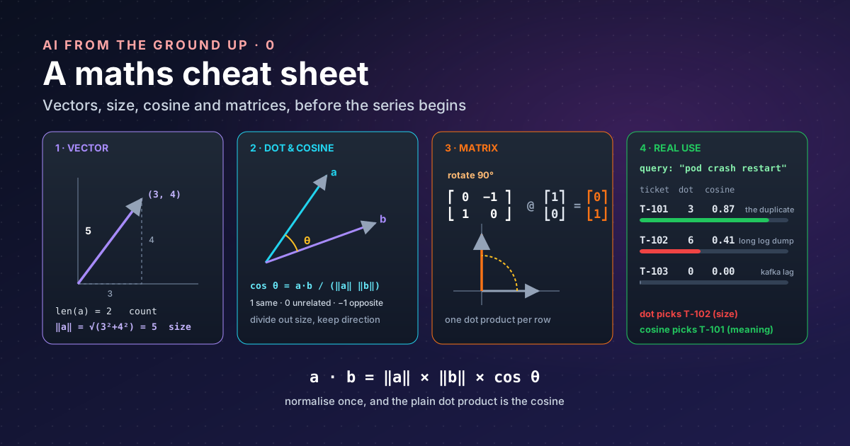
| Size, also called magnitude or norm, written ‖a‖ | How long the arrow is: square each number, add them, take the square root | √(3² + 4²) = 5 | np.linalg.norm(a) |
The size is Pythagoras: the arrow to (3, 4) is the long side of a right-angled triangle with sides 3 and 4. When maths texts divide “by the length” of a vector, they always mean the size, never the count.
2. What you can do with vectors#
import numpy as np

a = np.array([3.0, 4.0])
b = np.array([1.0, 2.0])

print("a + b  =", a + b)                  # add position by position
print("2 * a  =", 2 * a)                  # scale every number
print("a . b  =", a @ b)                  # dot product: 3*1 + 4*2
print("len(a) =", len(a))                 # how many numbers (dimensions)
print("|a|    =", np.linalg.norm(a))      # size (norm): sqrt(3**2 + 4**2)

u = a / np.linalg.norm(a)                 # normalise: same direction, size 1
print("unit a =", u, "size", np.linalg.norm(u))
a + b = [4. 6.]
2 * a = [6. 8.]
a . b = 11.0
len(a) = 2
|a| = 5.0
unit a = [0.6 0.8] size 1.0| Operation | What it does | Picture |
|---|---|---|
Add a + b | Add matching positions | Put one arrow on the end of the other |
Scale 2 * a | Multiply every number | Same direction, twice as long |
Dot product a · b | Multiply matching positions, add the results: one number | Large when the arrows point the same way |
Normalise a / ‖a‖ | Divide by the size | Same direction, size exactly 1 (a unit vector) |
3. Cosine similarity: comparing direction only#
The dot product mixes two things together: how much two arrows point the same way, and how big they are. Geometry gives the exact relationship:
a · b = ‖a‖ × ‖b‖ × cos θ, where θ (theta) is the angle between the arrows
Divide both sides by the two sizes and only the angle is left:
cosine similarity = a · b / (‖a‖ × ‖b‖) = cos θ
That is the whole reason for the division: it cancels the sizes so you compare direction alone. Wikipedia puts it the same way: the result depends only on the angle, so scaling a vector does not change it.
| Angle | cos θ | Read it as |
|---|---|---|
| 0° | 1 | same direction: as similar as it gets |
| 90° | 0 | at right angles: unrelated |
| 180° | −1 | opposite directions |
Here is why the division matters, using the toy word vectors from part 1. “Node” is a Kubernetes word with nothing in common with “cat”. Make the node arrow ten times bigger without turning it:
import numpy as np

cat  = np.array([0.9, 0.8, 0.1, 0.0])
dog  = np.array([0.8, 0.9, 0.2, 0.0])
node = np.array([0.1, 0.0, 0.8, 0.9])
big_node = 10 * node                      # same direction, ten times the size

def cosine(a, b):
    return a @ b / (np.linalg.norm(a) * np.linalg.norm(b))

for name, other in [("dog", dog), ("node", node), ("10 x node", big_node)]:
    print(f"cat vs {name:<9}  dot {cat @ other:5.2f}   cosine {cosine(cat, other):.2f}")
cat vs dog dot 1.46 cosine 0.99
cat vs node dot 0.17 cosine 0.12
cat vs 10 x node dot 1.70 cosine 0.12The raw dot product now says “cat” is closer to the big “node” (1.70) than to “dog” (1.46), which is nonsense. Cosine is not fooled: 0.12 either way.
4. Matrix: a machine that transforms vectors#
A matrix is a rectangular grid of numbers. Its shape is written rows × columns: a 3 × 4 matrix has 3 rows of 4 numbers.
Multiplying a matrix by a vector takes one dot product per row: each row is dotted with the vector, and the answers form a new vector. That is the useful way to think of a matrix: a machine that takes a vector in and gives a transformed vector out. 3Blue1Brown’s lesson shows this visually: the columns of the matrix record where the basic arrows land.
import numpy as np

v = np.array([1.0, 0.0])                  # an arrow pointing right

rotate = np.array([[0.0, -1.0],
                   [1.0,  0.0]])          # turn 90 degrees anticlockwise
stretch = np.array([[2.0, 0.0],
                    [0.0, 0.5]])          # double x, halve y

print("rotate  @ v =", rotate @ v)
print("stretch @ [1, 1] =", stretch @ np.array([1.0, 1.0]))
print("both, one matrix:\n", stretch @ rotate)   # two steps fused into one

W = np.random.default_rng(0).normal(size=(3, 4))  # a tiny "layer": 4 numbers in, 3 out
x = np.ones(4)
print("shape", W.shape, "@", x.shape, "->", (W @ x).shape)
rotate @ v = [0. 1.]
stretch @ [1, 1] = [2. 0.5]
both, one matrix:
[[ 0. -2. ]
[ 0.5 0. ]]
shape (3, 4) @ (4,) -> (3,)Three rules cover almost everything in the series:
- Shapes must line up. A (3 × 4) matrix needs a vector of 4 numbers and returns 3. The inner numbers must match: (3 × 4) @ (4) → (3).
- Multiplying two matrices chains two transformations into one matrix, as
stretch @ rotateshows. - Transpose (written Aᵀ) flips a matrix so rows become columns. Attention in part 1 uses it to line up shapes so every token can be dotted with every other.
A layer of a neural network is exactly the last line of that example: a matrix of learned numbers (the weights) that turns one vector into another. An LLM is billions of those numbers arranged in many such matrices.
5. Why turn things into vectors at all?#
This is the question behind the whole series. Three reasons:
- Computers compare numbers, not meanings. A program cannot tell that “pancake” and “crêpe” are alike by looking at the letters. Turn each into a vector and similarity becomes arithmetic.
- The obvious encoding is wasteful and says nothing. The simplest way to number 5,000 menu items is a one-hot vector: 5,000 positions, all 0 except a single 1. Google’s embeddings course uses exactly this example and points out the cost: huge inputs need huge numbers of weights, more data and more memory. Worse, every pair of one-hot vectors is at right angles (cosine 0), so “pancake” is as far from “crêpe” as from “shawarma”.
- A learned vector (an embedding) puts similar things near each other. In an embedding, items used in similar contexts end up closer together, with a few hundred or thousand numbers instead of thousands of mostly zeros. Once everything is a vector, one cheap operation (the dot product) compares anything with anything, and that operation is what GPUs are built to do billions of times a second (part 3).
And why the second transformation, normalising? Because size usually measures something you do not want to compare: how long a document is, how often a word appears, how popular an item is. Divide it out once and only the direction, the meaning, remains.
6. Where cosine similarity earns its keep#
The place I meet cosine most is search. In Elasticsearch, a dense_vector field
defaults to cosine similarity,
and the documentation explains a neat trick: “during indexing Elasticsearch automatically normalizes vectors with
cosine similarity to unit length”, which lets it use the plain dot product internally, “which is more efficient”.
PostgreSQL’s pgvector gives the same advice the other way round: if your
vectors are already normalised, “use inner product for best performance”.
A small, real-shaped example shows why cosine is the right choice for search. A new ticket says “pod crash restart”. Which old ticket is the duplicate? Each ticket becomes a vector of word counts, one position per word:
from collections import Counter
import numpy as np

tickets = {
    "T-101": "pod crash restart loop",
    "T-102": "pod pod pod pod pod pod disk full disk full disk full disk full node log dump",
    "T-103": "kafka consumer lag growing",
}
query = "pod crash restart"

vocab = sorted({w for text in [query, *tickets.values()] for w in text.split()})

def to_vector(text):                      # word counts: one position per vocabulary word
    counts = Counter(text.split())
    return np.array([counts[w] for w in vocab], dtype=float)

def cosine(a, b):
    return a @ b / (np.linalg.norm(a) * np.linalg.norm(b))

q = to_vector(query)
print(f"{'ticket':<6}  {'dot':>4}  {'cosine':>6}")
for tid, text in tickets.items():
    t = to_vector(text)
    print(f"{tid:<6}  {q @ t:4.0f}  {cosine(q, t):6.2f}")

unit = lambda v: v / np.linalg.norm(v)    # normalise once, when storing
print("unit dot T-101:", round(unit(q) @ unit(to_vector(tickets["T-101"])), 2))
ticket dot cosine
T-101 3 0.87
T-102 6 0.41
T-103 0 0.00
unit dot T-101: 0.87The dot product picks T-102, a long log dump about a full disk, simply because it repeats “pod” six times. Cosine picks T-101, the real duplicate. The last line is the Elasticsearch trick in miniature: normalise once when you store a vector, and the plain dot product is the cosine. Real systems use embeddings from a model rather than word counts, but the comparison is exactly this.
| Use | What is compared | Why cosine fits |
|---|---|---|
| Semantic search and RAG | A question’s embedding against stored text chunks | Matches meaning, not wording or length |
| Duplicate detection | New tickets, bug reports or alerts against old ones | A short and a long report of the same problem should match |
| Document similarity | Word-count or TF-IDF vectors | It normalises for document length |
| Recommendations | A user’s embedding against item embeddings | Stops popular items winning on size alone |
| Grouping (clustering) | Texts or users against each other | Groups by topic, not by volume |
When not to use it#
- When size carries meaning. Positions, prices and sensor readings need ordinary straight-line (Euclidean) distance. And in recommendations, Google’s recommendation course notes that the dot product is “sensitive to the norm of the embedding”: frequent items get large norms. Use it if you want popularity to count, knowing that popular items “may end up dominating the recommendations”.
- When vectors are already normalised. Then cosine and dot product give the same answer, so use the cheaper dot product.
- Inside a model’s attention. Part 1 shows attention using the raw dot product, scaled by √d rather than divided by the sizes. There the size is a signal the model learns to use.
- As a distance for maths that needs a true distance. “1 − cosine” is often called cosine distance, but it is not a true distance metric (it breaks the triangle rule). Most tools handle this for you.
Notation at a glance#
| You will see | Say it | Means | NumPy |
|---|---|---|---|
x | x | a scalar (one number) | x = 2.0 |
a, [a₁, a₂, …] | vector a | a list of numbers; aᵢ is the i-th one | np.array([...]) |
‖a‖ | norm (size) of a | √(a₁² + a₂² + …) | np.linalg.norm(a) |
a · b | a dot b | a₁b₁ + a₂b₂ + … | a @ b |
cos θ | cosine of theta | a · b / (‖a‖ ‖b‖) | (the function above) |
A, m × n | matrix A, m by n | grid with m rows and n columns | A.shape |
Aᵀ | A transpose | rows and columns swapped | A.T |
A · B, AB | A times B | matrix multiplication | A @ B |
Σ | sum | add up a list | np.sum(x) |
√d | root d | square root of d (the vector size in attention) | np.sqrt(d) |
eˣ | e to the x | exponential, used by softmax (part 1) | np.exp(x) |
log x | log of x | the natural logarithm, used by the loss (part 2) | np.log(x) |
∂L/∂w | dee L by dee w | how much L changes when w moves a little: a slope (part 1) | (computed by PyTorch) |
10²⁵ | ten to the 25 | 1 followed by 25 zeros (part 4) | 1e25 |
Takeaways#
- A vector is a list of numbers describing one thing, best pictured as an arrow.
- “Length” means size (norm), not count: square, add, square-root.
- The dot product measures alignment × size; cosine divides the sizes out and leaves direction alone.
- A matrix transforms vectors, one dot product per row; a neural network layer is one matrix of learned numbers.
- We turn things into vectors so that meaning becomes arithmetic, and normalise them so that length, frequency or popularity does not drown out meaning. That is why cosine powers search, duplicate detection and RAG.
Keywords#
| Term | What it means |
|---|---|
| Scalar | A single number. |
| Vector | An ordered list of numbers describing one thing; pictured as an arrow. |
| Dimension | How many numbers a vector has. |
| Norm / magnitude / size | How long the arrow is: the square root of the sum of the squares. |
| Unit vector | A vector of size 1. |
| Normalise | Divide a vector by its size, keeping only its direction. |
| Dot product | Multiply matching positions and add: large when two vectors point the same way. |
| Cosine similarity | Dot product divided by both sizes: 1 same direction, 0 unrelated, −1 opposite. |
| Euclidean distance | Ordinary straight-line distance between two points. |
| Matrix | A grid of numbers; multiplying a vector by it transforms the vector. |
| Shape | A matrix’s rows × columns. |
| Transpose | Flip a matrix so rows become columns. |
| Weights | The learned numbers inside a model’s matrices. |
| One-hot vector | All zeros except a single 1 marking which item it is. |
| Embedding | A learned vector that places similar things close together. |
| TF-IDF | Word counts weighted so common words count less; a classic document vector. |
| RAG | Retrieval-augmented generation: find relevant text by similarity, then give it to an LLM. |
References#
- NumPy documentation: NumPy; the array library used in the examples
- Cosine similarity: Wikipedia; definition, range, scale independence, length normalisation in text mining, cosine distance not being a metric
- sklearn.metrics.pairwise.cosine_similarity: scikit-learn; the normalised dot product formula and its equivalence to the dot product on normalised data
- Linear transformations and matrices: 3Blue1Brown; a matrix as a transformation whose columns record where the basic arrows land
- Embeddings: Google Machine Learning Crash Course; one-hot vectors, the 5,000 meal example and their cost
- Embedding space and static embeddings: Google Machine Learning Crash Course; similar items sit closer together
- Candidate generation overview: Google Recommendation Systems course; cosine vs dot product vs Euclidean distance and the effect of popular items
- Dense vector field type: Elastic documentation;
cosineas the default similarity and normalisation at index time - pgvector: pgvector project; distance operators and inner product for normalised vectors
Next in the series: part 1, the maths behind an LLM, where these pieces become attention, softmax and training.